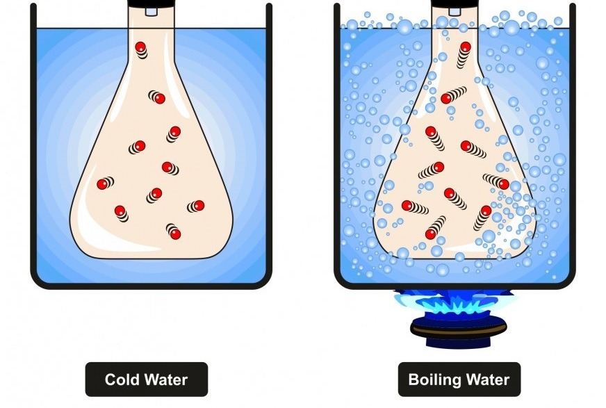
We aim to use computer simulations to model some aspect of reality. Most experiments that we try to match are performed under constant temperature and pressure, so we also want our simulations to reflect the same constant temperature and pressure.* Just as you have a thermostat in your home to regulate ambient temperature, e.g., heating in the wintertime or air conditioning in the summertime, there are thermostats in MD simulations to regulate the temperature of the system. Without assuming you’ve had formal coursework in statistical mechanics, I’ll briefly describe four flavors of thermostats, and some variants thereof:
- Velocity rescaling
- Nosé–Hoover
- Langevin
- Andersen
The velocity rescaling method, well, scales velocities
In an MD simulation, the coordinates and velocities (momenta) of all components in the system are propagated in time using Newton’s equations of motion. (see “What are molecular dynamics simulations?”) From basic physics, we know that kinetic energy directly depends on velocities via:
[math]KE=\frac{1}{2}mv^2[/math]
Then, from the equipartition theorem, the temperature of the system is related to the average kinetic energy to velocities via the time average of the kinetic energy [2]. For the translational degrees of freedom (e.g., motion along x, y, z), this can be written:
[math]KE_{avg}=\frac{3}{2}k_BT[/math]
where kB is the Boltzmann constant. From setting both expressions equal to each other, we can see that by adjusting velocities we can manipulate the temperature of the system.
[math]\langle\frac{1}{2}mv^2\rangle=\frac{3}{2}k_BT[/math]
Therefore, the velocity scaling method simply scales the velocities at every time step by the factor [ref. 1, Appendix A]:
[math]\lambda = \sqrt{\frac{T_{req}}{T_{curr}}}[/math]
where Tcurr is the current temperature calculated from the kinetic energy, and Tdes is the desired temperature.
- Advantages:
- Straightforward approach to implement
- Fine to use in warm up phase
- Disadvantages:
- Not time reversible
- No “natural” temperature fluctuations
- Could lead to artificial temperature differences among system components, e.g., “hot solvent, cold solute”, in which the temperature of the solute could be less than the temp of the solvent, despite overall system temperature being the desired value.
- Does not correspond to a particular statistical ensemble [3]. In overly simplistic terms, this means the system doesn’t correspond to a particular state in the real world, such as a state with fixed number of particles, at constant temperature and pressure.
The Berendsen thermostat is another algorithm that maintains temperature by scaling the velocities at each time step. In this case, the system is coupled to an external heat bath, which adds or removes heat as necessary. The velocity is scaled to have the temperature’s rate of change be proportional to the temperature difference between bath and system [ref. 1, Appendix B]. This method does allow fluctuations around the desired temperature.
The Nosé–Hoover method uses an extra degree of freedom as thermal reservoir
[details TBD]
The Langevin method balances random noise and friction
[details TBD]
The Andersen method randomizes velocities
For the Andersen method, the equations of motion include an extra term for stochastic (random) collisions. At regular intervals, particles are chosen at random for velocity reassignment. The new velocity is sampled from the Maxwell-Boltzmann distribution. This method is equivalent to having the system be coupled to a heat bath that imposes the desired temperature by randomly emitting “thermal particles.” In between collisions, the system is simulated with constant energy, which we interpret as a microcanonical ensemble. A trajectory with Andersen temperature regulation can therefore be seen as a series of microcanonical simulations, each conducted with a slightly different energy, and all together having a Gaussian distribution.
- Advantages
- Samples from canonical ensemble, with constant number of particles, volume, and temperature
- Disadvantages
- Trajectory is not smooth due to rescaling jumps
- Dynamics of system don’t represent physical reality
There’s a variant of the Andersen thermostat called the Lowe-Andersen thermostat.[4]
[details TBD]
Closing remarks
These are just four of the number of methods out there to regulate temperature in molecular dynamics simulations. In practice, I’ve commonly seen the Langevin, Lowe-Andersen, and Nosé–Hoover thermostats. If you want a more general view, I’d suggest going through current papers on projects that utilize molecular dynamics simulations, and check out their methods sections.
Footnotes
*There are other purposes of temperature regulation besides matching experimental conditions. For example, we can apply simulated annealing algorithms, used for searching conformational space and for structural determination from NMR and X-ray data. [1]
Additional resources
- Among NVT and NPT ensemble which one is preferable during MD simulation?
- Thermostats in Molecular Dynamics Simulations
- Stochastic NVT Thermostats
Appendices
A. Short derivation of scaling factor for velocity scaling
B. Short derivation of scaling factor for Berendsen thermostat
References
- Molecular Modelling: Principles and Applications. Leach. p. 383.
- Equipartition of energy
- Thermodynamic ensembles
- Advantages of a Lowe-Andersen thermostat in molecular dynamics simulations
